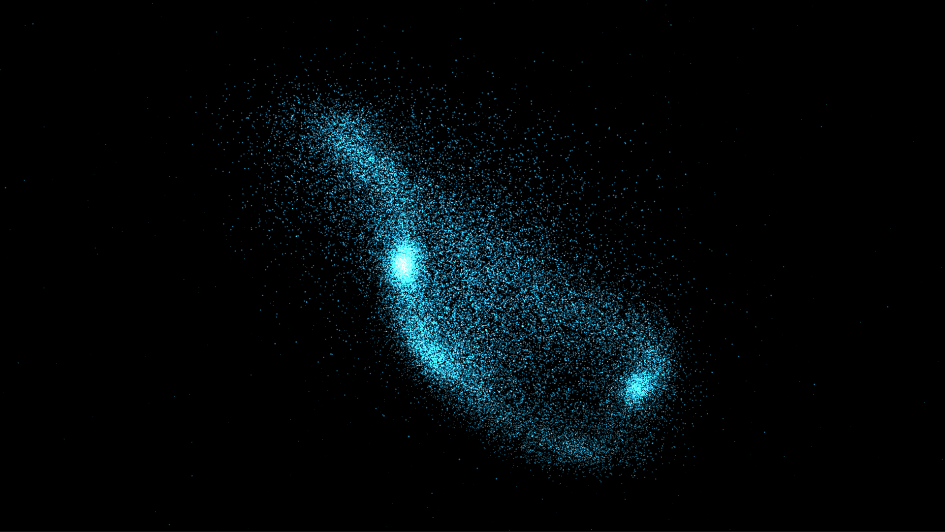
Figure 2.1: Result
In this chapter, we will explain the GPU implementation method of Gravitational N-Body Simulation, which is a method of simulating the movement of celestial bodies existing in outer space.
Figure 2.1: Result
The corresponding sample program is
https://github.com/IndieVisualLab/UnityGraphicsProgramming3
"Assets / NBodySimulation".
Simulations that calculate the interaction of N physical objects are collectively called N-Body simulations. There are many types of problems using N-Body simulation, and in particular, the problem of dealing with a system in which celestial bodies scattered in outer space attract each other by gravity to form a unit is called a gravity multisystem problem. I will. The algorithm explained in this chapter corresponds to this, and it means to solve the equation of motion of the gravitational multisystem using N-Body simulation.
In addition to the gravity multisystem problem, N-Body simulation is also available.
It is applied in a wide range of fields, from small to magnificent.
Let's see what kind of mathematical formulas we will solve immediately.
The gravitational multisystem problem can be simulated by calculating the universal gravitational equation, which is a familiar equation for those who are taking high school physics, for all celestial bodies in space. However, in high school physics, I think that it was learned with such a description because it deals only with objects that are in a straight line.
Where f is the universal gravitational force, G is the gravitational constant, M and m are the masses of the two objects, and r is the distance between the objects. Of course, this can only determine the magnitude of the force (scalar amount) between two objects .
In this implementation, it is necessary to consider the movement in the 3D space inside Unity, so a vector quantity indicating the direction is required. Therefore, in order to find the vector of the force generated between two celestial bodies ( i, j ), the equation of universal gravitational force is described as follows.
Here, \ mbox {\ boldmath $ f $} _ {ij} is the vector of the force that the object i receives from the object j, m_i and m_j are the masses of the two objects, and r_ {ij} is the object i from the object j. Direction vector to. On the left side of the right side, the magnitude of the force is calculated in the same way as the equation of universal gravitational force that first appeared, and it is vectorized by multiplying the unit vector in the direction of receiving the force on the right side of the right side.
missing image: takao / vec
Figure: Meaning of formula
Furthermore, if the magnitude of the force that one object ( i ) receives from all the surrounding objects, not between two objects, is \ mbox {\ boldmath $ F $} _ {i} , it can be calculated as follows. ..
As shown in the formula, the force received from the surrounding celestial bodies can be calculated by taking the sum of all universal gravitational forces.
Also, to simplify the simulation, the equation can be rewritten using the Softening factor \ varepsilon as follows.
This makes it possible to ignore collisions even if the celestial bodies come to the same position (even if they calculate themselves, the result in Sigma will be 0 ).
Next, using the second law of motion m \ mbox {\ boldmath $ a $} = \ mbox {\ boldmath $ f $}, we will convert the force vector into the acceleration vector. First, we transform the second law of motion into the following equation.
Next, by substituting the above transformation equation into the equation of motion of the gravitational multisystem and rewriting it, the acceleration received by the celestial body can be calculated.
The simulation is now ready. Now that we were able to express the gravitational multisystem problem with mathematical formulas, how can we incorporate these mathematical formulas into our program? I would like to explain it firmly in the next section.
The above equation (\ ref {eq: newton}) is classified as a differential equation among the equations . Because, in the physical world, the relationship between position, velocity, and acceleration is as shown in the following image, and since acceleration is the second derivative of the position function, it is called a differential equation as it is.
Figure 2.2: Relationship between position, velocity, and acceleration
There are various methods for solving differential equations with a computer, but the most common one is the algorithm called the difference method . Let's start with a review of differentiation.
First, let's review the definition of mathematical differentiation. The derivative of the function f (t) is defined by the following equation.
Since it is difficult to understand what is shown by the formula alone, it becomes as follows when replaced with a graph.
Figure 2.3: Forward difference
You already know that the differential value of the function is the slope of the graph at t_n . After all, this graph shows the state that \ Delta t is made infinitely small to calculate the slope, and you can see that it represents the formula (\ ref {eq: delta}) itself. think.
You cannot handle "infinity" as a numerical value on a computer. Therefore, we will approximate it with a finite \ Delta t that is as small as possible . With that in mind, if we rewrite the definition of differentiation to difference, we get the following equation.
It's a shape that has taken the limit as it is. I think it's okay to recognize that "an infinitesimal \ Delta t cannot be represented on a computer, so stop at a certain size \ Delta t to approximate it."
Here, the physical representation of Figure 2.2 above is as follows.
Figure 2.4: Relationship between position, velocity, and acceleration (mathematical formula)
That is, the formula (\ ref {eq: diffuse}) is compared to Figure 2.4 as follows:
Furthermore, when the formulas (\ ref {eq: x}) and (\ ref {eq: v}) are combined, the result is as follows.
This formula means that " the position coordinates after \ Delta t seconds from the current time t can be calculated if the acceleration and velocity of the current time are known." This is the basic idea when simulating with the finite difference method. In addition, the expression of such a differential equation using the difference method is called a difference equation (recurrence formula) .
When actually performing real-time simulation by the difference method, it is common to set the minute time \ Delta t (time step) to the drawing time of one frame (1/60 second at 60 fps).
Now, let's get into the implementation. The corresponding scene will be "SimpleNBodySimulation.unity".
First of all, we define the data structure of celestial particles. Looking at the equation (\ ref {eq: delta}), we can see that the physical quantities that one celestial body should have are "position, velocity, mass". Therefore, it seems good to define the following structure.
Body.cs
public struct Body
{
  public Vector3 position;
  public Vector3 velocity;
  public float mass;
}
Next, set the number of particles you want to generate from the inspector, and secure a buffer for that number. Separate buffers for reading and writing to prevent data race conditions.
In addition, the number of bytes per structure can be obtained with the "Marshal.SizeOf (Type t)" function in the "System.Runtime.InteropServices" namespace.
SimpleNBodySimulation.cs
void InitBuffer()
{
  // Create buffer (for Read / Write) → Conflict prevention
  bodyBuffers = new ComputeBuffer[2];

    // Each element creates a buffer of Body structure for the number of particles
  bodyBuffers[READ] = new ComputeBuffer(numBodies,
    Marshal.SizeOf(typeof(Body)));

  bodyBuffers[WRITE] = new ComputeBuffer(numBodies,
    Marshal.SizeOf(typeof(Body)));
}
Then place the particles in space. First, create an array for the particles and give each element an initial value of the physical quantity. In the sample, the inside of the sphere was randomly sampled as the initial position, the velocity was 0, and the mass was randomly given.
Finally, set the buffer for the created array and you are ready * 1 .
[* 1] * For look adjustment, we have prepared a variable that can scale the position coordinates, but you do not have to worry because it has already been adjusted.
SimpleNBodySimulation.cs
void DistributeBodies()
{
  Random.InitState(seed);

  // For look adjustment
  float scale = positionScale
                * Mathf.Max(1, numBodies / DEFAULT_PARTICLE_NUM);

  // Prepare an array to set in the buffer
  Body[] bodies = new Body[numBodies];

  int i = 0;
  while (i < numBodies)
  {
    // Sampling inside the sphere
    Vector3 pos = Random.insideUnitSphere;

    // set in an array
    bodies[i].position = pos * scale;
    bodies[i].velocity = Vector3.zero;
    bodies[i].mass = Random.Range(0.1f, 1.0f);


    i++;
  }

  // Set the array in the buffer
  bodyBuffers[READ].SetData(bodies);
  bodyBuffers[WRITE].SetData(bodies);

}
Finally, we will actually move the simulation. The following code is the part that is executed every frame.
First, set the value in the constant buffer of ComputeShader. For \ Delta t of the difference equation, use "Time.deltaTime" provided by Unity. In addition, due to the implementation of GPU, the number of threads and the number of thread blocks are also transferred.
After the calculation is completed, the calculation result of the simulation is stored in the buffer for writing, so the buffer is replaced in the last line so that it can be used as the buffer for reading in the next frame.
SimpleNBodySimulation.cs
void Update()
{
// Transfer constants to compute shader
// Δt
NBodyCS.SetFloat ("_ DeltaTime", Time.deltaTime);
// Speed attenuation rate
NBodyCS.SetFloat("_Damping", damping);
// Softening factor
NBodyCS.SetFloat("_SofteningSquared", softeningSquared);
// Number of particles
NBodyCS.SetInt("_NumBodies", numBodies);
// Number of threads per block
NBodyCS.SetVector("_ThreadDim",
new Vector4(SIMULATION_BLOCK_SIZE, 1, 1, 0));
// Number of blocks
NBodyCS.SetVector("_GroupDim",
new Vector4(Mathf.CeilToInt(numBodies / SIMULATION_BLOCK_SIZE), 1, 1, 0));
// Transfer the buffer address
NBodyCS.SetBuffer(0, "_BodiesBufferRead", bodyBuffers[READ]);
NBodyCS.SetBuffer(0, "_BodiesBufferWrite", bodyBuffers[WRITE]);
// Compute shader execution
NBodyCS.Dispatch(0,
Mathf.CeilToInt(numBodies / SIMULATION_BLOCK_SIZE), 1, 1);
// Swap Read / Write (conflict prevention)
Swap(bodyBuffers);
}
After the simulation calculation, issue an instance drawing instruction to the material that renders the particles. When rendering a particle, it is necessary to give the position coordinates of the particle to the shader, so transfer the calculated buffer to the shader for rendering.
ParticleRenderer.cs
void OnRenderObject ()
{
  particleRenderMat.SetPass (0);
  particleRenderMat.SetBuffer("_Particles"", bodyBuffers[READ]);

  Graphics.DrawProcedural(MeshTopology.Points, numBodies);
}
In N-Body simulation, it is necessary to calculate the interaction with all particles, so if it is calculated simply, the execution time will be O (n ^ 2) and performance cannot be achieved. Therefore, I will utilize the usage of Shared Memory described in Chapter 3 of UnityGraphicsProgramming Vol1.
Data in the same block is stored in shared memory, which speeds up I / O. The following is a conceptual diagram that resembles a thread block as a tile.
Figure 2.5: Tile concept
Here, the row is the global thread (DispatchThreadID) that is running, and the column is the particle that is being exhausted in the thread. It's like the columns you're running are shifting one by one to the right over time.
Also, the total number of tiles executed at the same time is (number of particles / number of threads in the group). In the sample, the number of threads in the block is 256 (SIMULATION_BLOCK_SIZE), so it is recognized that the tile content is actually 256x256 instead of 5x5.
All rows are running in parallel, but because they share data within the tile, they wait until all the columns running in the tile reach Sync (do not go to the right of the Sync layer). After reaching the Sync layer, the data of the next tile is reloaded into the shared memory.
Describe the constant buffer for receiving the input from the CPU in the Compute Shader.
Also, prepare a buffer for storing particle data. This time, the Body structure is summarized in "Body.cginc". It is convenient to put together cginc for things that are likely to be reused later.
Finally, make a declaration to use shared memory.
SimpleNBodySimulation.compute
#include "Body.cginc"

// constant
cbuffer cb {
        float   _SofteningSquared, _DeltaTime, _Damping;
        uint    _NumBodies;
        float4  _GroupDim, _ThreadDim;
};


// Particle buffer
StructuredBuffer<Body> _BodiesBufferRead;
RWStructuredBuffer<Body> _BodiesBufferWrite;

// Shared memory (shared within the block)
groupshared Body sharedBody[SIMULATION_BLOCK_SIZE];
Next, implement the tile.
SimpleNBodySimulation.compute
float3 computeBodyForce(Body body, uint3 groupID, uint3 threadID)
{

  uint start = 0; // start
  uint finish = _NumBodies;

  float3 acc = (float3)0;
  int currentTile = 0;

  // Execute for the number of tiles (number of blocks)
  for (uint i = start; i < finish; i += SIMULATION_BLOCK_SIZE)
  {
    // Store in shared memory
    // sharedBody [thread ID in block]
    // = _BodiesBufferRead [tile ID * total number of threads in block + thread ID]
    sharedBody[threadID.x]
      = _BodiesBufferRead[wrap(groupID.x + currentTile, _GroupDim.x)
        * SIMULATION_BLOCK_SIZE + threadID.x];

    // Group sync
    GroupMemoryBarrierWithGroupSync();

    // Calculate the effect of gravity from the surroundings
    acc = gravitation(body, acc, threadID);

    GroupMemoryBarrierWithGroupSync();

    currentTile ++; // Go to the next tile
  }

  return acc;

}
Put the image of the for loop in the code in the next image.
Figure 2.6: Tile ID for loop
Since we controlled the movement of the tile in the previous loop, we will implement the for loop in the tile this time .
SimpleNBodySimulation.compute
float3 gravitation(Body body, float3 accel, uint3 threadID)
{

  // 100% survey
  // Execute for the number of threads in the block
  for (uint i = 0; i < SIMULATION_BLOCK_SIZE;)
  {
    accel = bodyBodyInteraction(accel, sharedBody[i], body);
    i++;
  }

  return accel;
}
This completes the 100% survey in the tile. Also, at the timing after the return of this function, it waits until all the threads in the tile complete the process.
Then implement the expression (\ ref {eq: first}) as follows:
SimpleNBodySimulation.compute
// Calculation in Sigma
float3 bodyBodyInteraction(float3 acc, Body b_i, Body b_j)
{
  float3 r = b_i.position - b_j.position;

  // distSqr = dot(r_ij, r_ij) + EPS^2
  float distSqr = r.x * r.x + r.y * r.y + r.z * r.z;
  distSqr += _SofteningSquared;

  // invDistCube = 1/distSqr^(3/2)
  float distSixth = distSqr * distSqr * distSqr;
  float invDistCube = 1.0f / sqrt(distSixth);

  // s = m_j * invDistCube
  float s = b_j.mass * invDistCube;

  // a_i =  a_i + s * r_ij
  acc += r * s;

  return acc;
}
This completes the program for calculating the total acceleration.
Next, the coordinates and velocity of the particles in the next frame are calculated using the acceleration calculated so far.
SimpleNBodySimulation.compute
[numthreads(SIMULATION_BLOCK_SIZE,1,1)]
void CSMain (
        uint3 groupID: SV_GroupID, // Group ID
        uint3 threadID: SV_GroupThreadID, // Thread ID in the group
        uint3 DTid: SV_DispatchThreadID // Global Thread ID
) {

        // Current global thread index
        uint index = DTid.x;

        // Read particles from buffer
        Body body = _BodiesBufferRead[index];

        float3 force = computeBodyForce(body, groupID, threadID);

        body.velocity + = force * _DeltaTime;
        body.velocity *= _Damping;

        // Difference
        body.position + = body.velocity * _DeltaTime;

        _BodiesBufferWrite[index] = body;

}
The position coordinates of the celestial body have been updated. This completes the simulation of the movement of the celestial body!
In this section, I would like to supplement the drawing method of GPU particles, which was insufficiently explained in the previous article * 2 .
[* 2] The same particle rendering is performed in "Unity Graphics Programming Vol.1-Chapter 5 Fluid Simulation by SPH Method".
A billboard is a simple planar object that always faces the camera. It is no exaggeration to say that most particle systems in the world are implemented by billboards. In order to implement the billboard simply, we need to make good use of the view transformation matrix.
The view transformation matrix contains numerical information that returns the camera position and rotation to the origin. In other words, by multiplying all the objects in space by the view transformation matrix, it is transformed into a coordinate system with the camera as the origin.
Therefore, for a billboard that has the characteristic of facing the direction of the camera, it seems that the inverse matrix of the view transformation matrix containing only the rotation information should be multiplied as the model transformation matrix. (Although it will be described later, it is difficult to understand, so the illustration is shown in Figure 2.8 .)
First of all, create a Quad mesh to draw the particles. This can be easily achieved by extending one vertex to a Quad parallel to the xy plane with a geometry shader * 3 .
[* 3] For a detailed explanation of geometry shaders, see UnityGraphicsProgramming Vol.1 "Growing grass with geometry shaders".
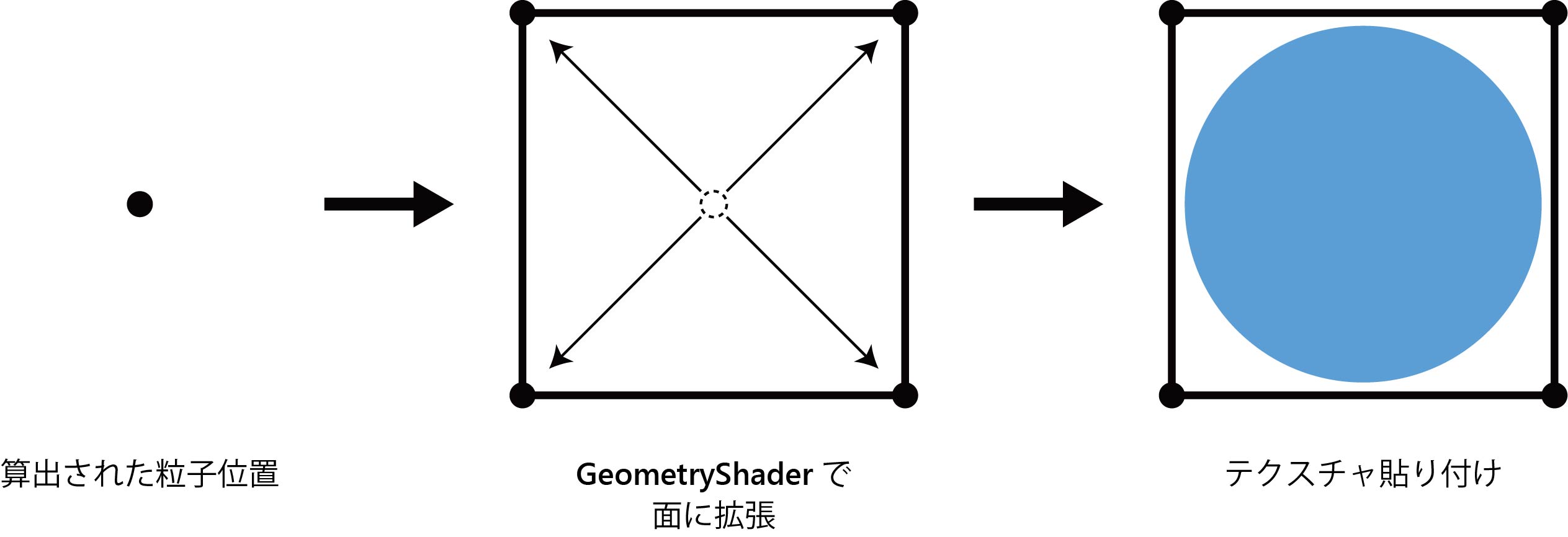
Figure 2.7: Quad extension with Geometry Shader
If you give this quad an inverse matrix * 4 that cancels the translation component of the view transformation matrix as a model transformation matrix, you can create a quad that faces the camera on the spot.
[* 4] Since it is known that the inverse matrix of the view transformation matrix can be simply transposed, it is implemented here by transposing.
I don't know what you're talking about, so here's an explanatory diagram.
Figure 2.8: How the billboard works
Furthermore, by applying a view and projection matrix to the billboard facing the camera, it can be converted to the coordinates on the screen. The shader that implements these is shown below.
ParticleRenderer.shader
[maxvertexcount(4)]
void geom(point v2g input[1], inout TriangleStream<g2f> outStream) {
  g2f o;

  float4 pos = input[0].pos;

  float4x4 billboardMatrix = UNITY_MATRIX_V;

  // Take out only the rotating component
  billboardMatrix._m03 = billboardMatrix._m13 =
    billboardMatrix._m23 = billboardMatrix._m33 = 0;

  for (int x = 0; x < 2; x++) {
    for (int y = 0; y < 2; y++) {
      float2 uv = float2(x, y);
      o.uv = uv;

      o.pos = pos
        + mul(transpose(billboardMatrix), float4((uv * 2 - float2(1, 1))
        * _Scale, 0, 1));

      o.pos = mul(UNITY_MATRIX_VP, o.pos);

      o.id = input[0].id;

      outStream.Append(o);
    }
  }

  outStream.RestartStrip();
}
Let's see the result of the above simulation.
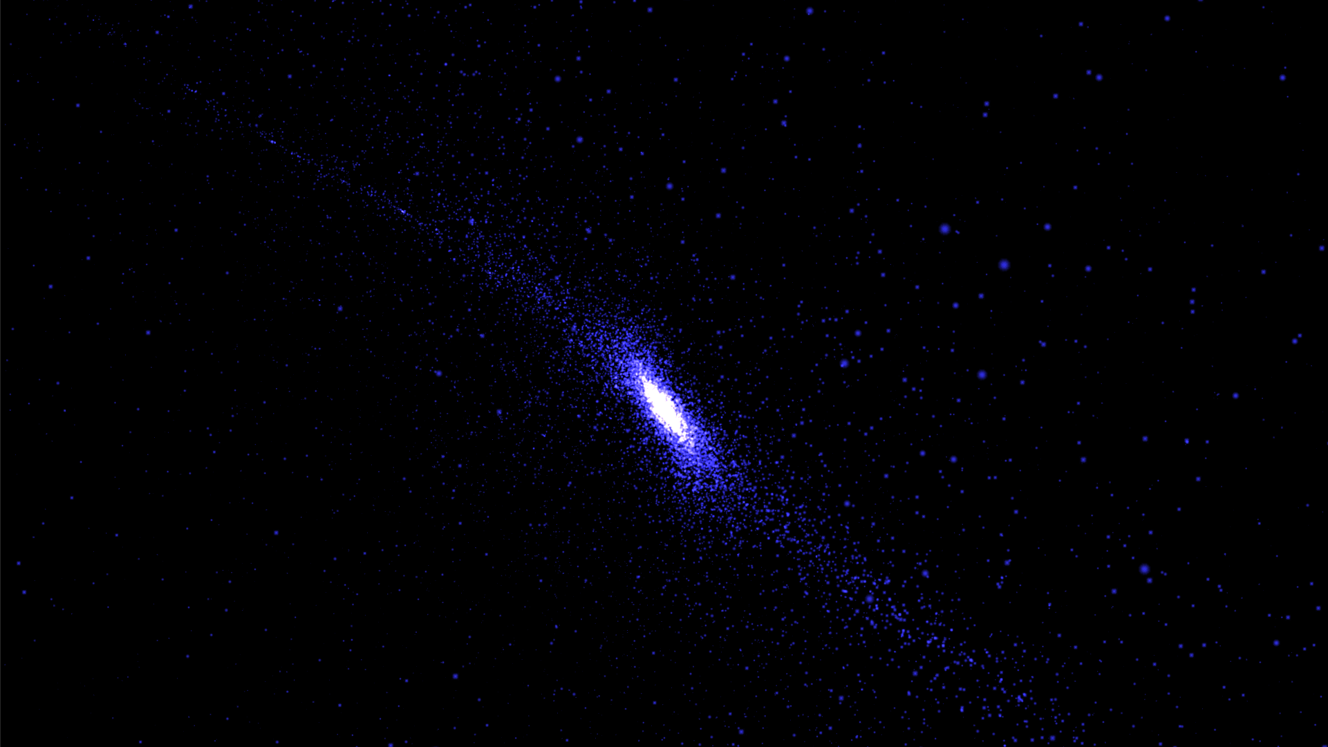
Figure 2.9: Simulation results (feeling of korejanai ...)
Looking at the movement, all the particles are gathered in the center, which is not visually interesting. Therefore, we will add some ideas in the next section.
The corresponding scene is "NBodySimulation.unity". Even if it is a device, there is only one line to change, and the tile calculation part will be cut off in the middle as follows.
NBodySimulation.compute
float3 computeBodyForce(Body body, uint3 groupID, uint3 threadID)
{
  ・・・

  uint finish = _NumBodies / div; // Cut in the middle

  ・・・

}
As a result, the calculation of the interaction is discarded in the middle without being exhausted, but as a result, it is not affected by all the particles, so some particle lumps are generated and aggregated into one point. Will never happen.
Then, the interaction between the parts of multiple masses produces a more dynamic movement as shown in Figure 2.1 at the beginning .
In this chapter, we explained the GPU implementation method of Gravitational N-Body Simulation. From small atoms to the large universe, the potential of N-Body simulation is infinite. Why don't you try to create your own universe on Unity? I hope you can help me even a little!